this started with an embarrassingly simple question:
\[\sqrt{2} \quad \text{or} \quad \sqrt[3]{3}\]which one is bigger?
i was trying to do it using a first-order Taylor approximation instead of just putting both into a calculator, cause apparently i enjoy turning one-line questions into a whole thing.
for the cube root, my first instinct was
\[3 = 27-24\]so
\[\sqrt[3]{3} = \sqrt[3]{27-24} = 3\left(1-\frac{24}{27}\right)^{1/3}.\]using
\[(1+x)^{1/3}\approx1+\frac{x}{3},\]i got
\[\sqrt[3]{3}\approx\frac{19}{9}\approx2.11.\]which is obviously horrible. the actual value is around \(1.442\).
i had expanded way too far away from the point where the approximation was supposed to be useful. if i rewrite it so the perturbation is small,
\[\sqrt[3]{3} = \frac32\left(1-\frac19\right)^{1/3},\]the same first-order idea gives about \(1.444\), which is excellent.
nothing surprising so far.
but the bad approximation bothered me, cause even though \(2.11\) is hilariously wrong as an approximation to \(1.442\), it can still answer the question i actually asked.
i did not care about the values.
i cared about
\[\sqrt[3]{3}>\sqrt2?\]and that is a different problem.
wrong numbers, right answer
using equally lazy first-order choices, i can get
\[\sqrt[3]{3}\approx2.11 \qquad\text{and}\qquad \sqrt2\approx1.50.\]the true numbers are
\[1.442\qquad\text{and}\qquad1.414.\]the estimates are bad, but both comparisons say the cube root is bigger. for the only question i asked, Taylor worked.
then the opposite can happen too. compare
\[A=\sqrt{1.1} \qquad\text{with}\qquad B=1.049.\]the true value is
\[\sqrt{1.1}\approx1.04881,\]so \(A<B\). but linearizing \(\sqrt{1+x}\) around zero gives
\[\sqrt{1+x}\approx1+\frac{x}{2},\]and at \(x=0.1\) that says \(A\approx1.05\), so Taylor says \(A>B\).
the numerical error here is tiny. it is just bigger than the even tinier separation between the values.
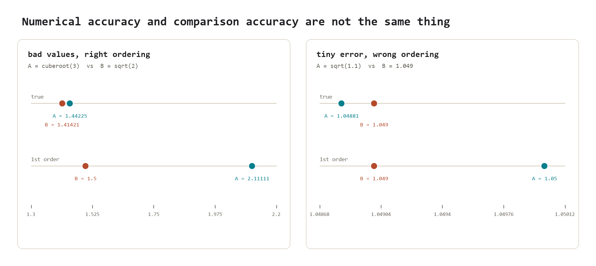
this is what sent me down the rabbit hole.
how wrong can Taylor be before it stops being right?
what actually causes a failure
suppose i have two true quantities
\[A,\qquad B\]and first-order approximations
\[\hat A,\qquad\hat B.\]write the true values as
\[A=\hat A+r_A, \qquad B=\hat B+r_B,\]where \(r_A\) and \(r_B\) are the remainders i threw away.
then
\[A-B=(\hat A-\hat B)+(r_A-r_B).\]let
\[D=A-B\]be the true difference. the part that matters is not the error in \(A\) or the error in \(B\) by itself. it is their difference:
\[R=r_A-r_B.\]because
\[\hat A-\hat B=D-R.\]if \(A>B\) and the true gap is
\[E=|A-B|=D>0,\]the comparison flips exactly when
\[E-R<0,\]or
\[\boxed{R>E}.\]thats the cleanest thing i got out of this whole thing.
a first-order comparison does not fail when the Taylor approximation becomes “bad”. it fails when the difference between the two errors becomes larger than the actual distance between the things being compared.
those are not the same thing.
a nicer variable than just the gap
the raw gap \(E\) tells me how hard the comparison is, but it does not tell me whether the error is pointed in a harmful direction.
so define
\[Q= \frac{ \operatorname{sgn}(A-B)(r_A-r_B) }{ |A-B| }.\]then the whole comparison collapses into one boundary:
\[Q<1 \quad\Longrightarrow\quad \text{ordering survives},\]and
\[Q>1 \quad\Longrightarrow\quad \text{sign flip}.\]i like this quantity a lot. it is asking:
how large is the harmful part of my Taylor error compared with the thing i am trying to distinguish?
if \(Q=0.01\), the error is nowhere near enough to matter. if \(Q=0.9\), im getting uncomfortable. if \(Q=1.01\), Taylor just crossed the decision boundary.
and \(Q\) can be very negative too. that is what happens when the errors are huge but push the comparison farther in the correct direction. the awful cube-root example lives there. the approximation is bad, but its badness helps the sign.
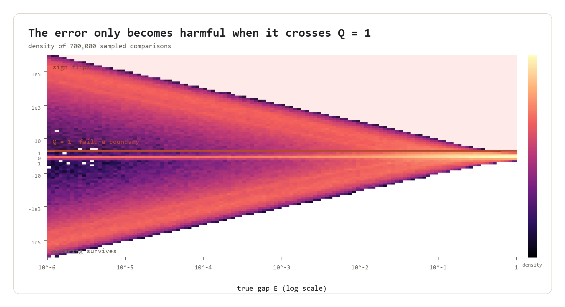
| the funnel shape is basically the whole story. as $E$ shrinks, the same remainder mismatch is divided by a smaller and smaller gap, so $ | Q | $ grows. if $Q$ grows upward past $1$, the approximation flips the sign; if it grows downward, the approximation may be numerically wrong but still preserve the ordering with an increasingly large margin. |
being close is not enough to make it fail
at this point i thought maybe the answer was just:
Taylor comparison works until the values get too close.
not quite.
take
\[f(x)=\sqrt{x}\]and compare \(f(1)\) with \(f(1+\epsilon)\) for some ridiculously small \(\epsilon>0\).
the first-order approximation around \(1\) is
\[T(x)=1+\frac{x-1}{2}.\]then
\[T(1+\epsilon)>T(1),\]and square root itself is increasing, so
\[\sqrt{1+\epsilon}>\sqrt1.\]this stays correct for \(\epsilon=10^{-3}\), \(10^{-50}\), or however stupidly small i want to make it.
the gap can approach zero and the comparison still never fails, cause the true function and the fixed tangent preserve the same ordering.
this caveat matters a lot: two values from the same monotone family, compared using the same fixed tangent with the correct slope sign, are order-correct. the interesting failures show up when i compare different families, different anchors, or otherwise different remainder structures.
so i tried the standard families
i used the usual suspects:
\[\sqrt{x},\quad \sqrt[3]{x},\quad x^{2/3},\quad e^x,\quad \log x,\quad \sin x,\quad \cos x.\]i aligned their expansion values at \(1\), sampled true outputs in the common range \(0.25\) to \(1.75\), and compared distinct family pairs. roots and log were expanded around input \(1\), exp and sin around \(0\), and cos around \(\pi/2\). the true gap \(E\) was sampled logarithmically from \(10^{-6}\) to \(1\) and the orientation was randomized.
then i did this three million times.
for every comparison i asked one yes/no question:
\[\operatorname{sign}(\hat A-\hat B) = \operatorname{sign}(A-B)?\]group those answers by the true gap and i get
\[p(E)=P(\text{correct ordering}\mid |A-B|\approx E).\]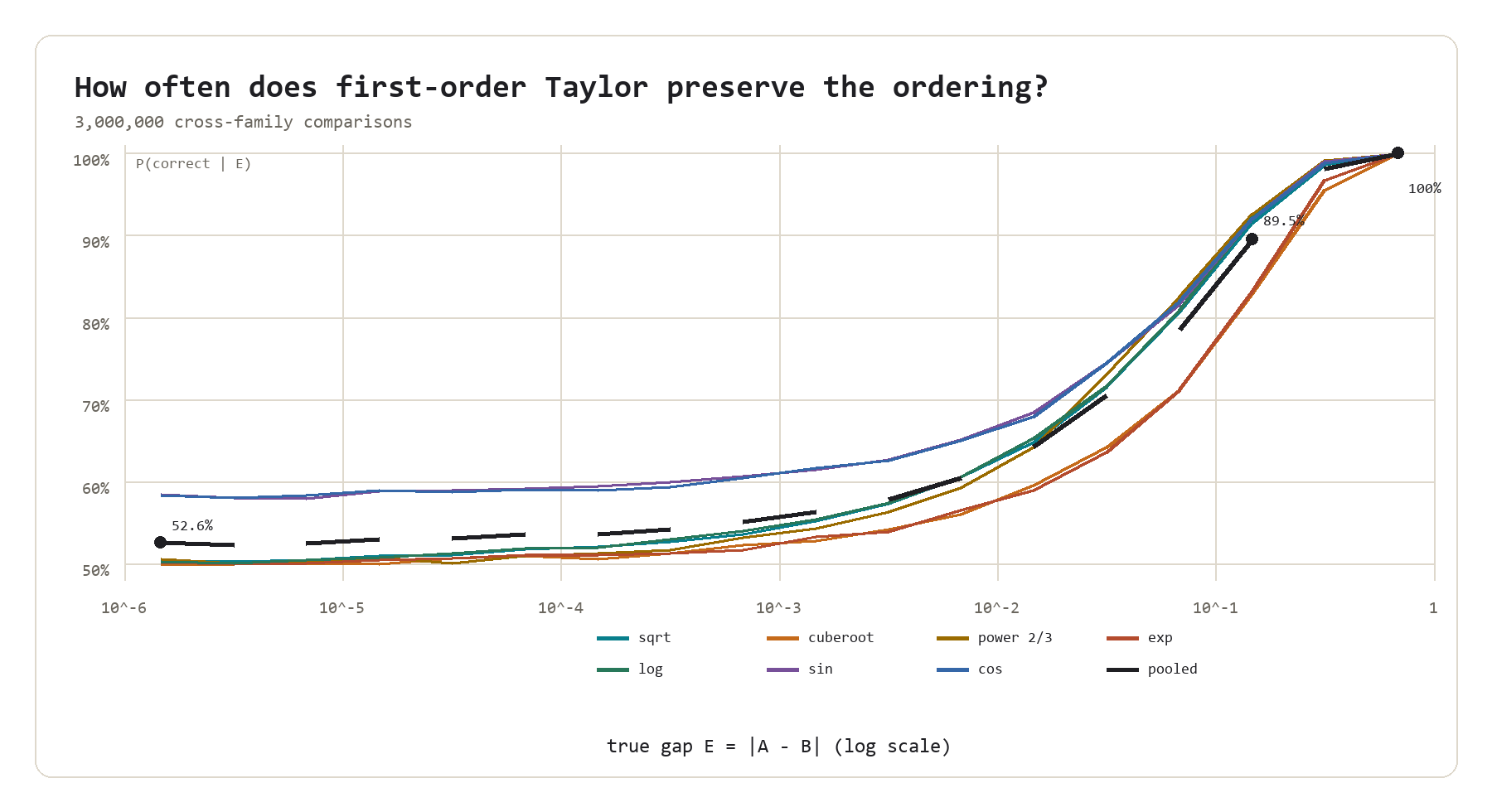
for this sampling rule, the pooled accuracy is about \(52.6\%\) near \(E=10^{-6}\), about \(60\%\) around \(E=0.007\), about \(90\%\) around \(E=0.15\), and basically perfect once the gap gets large enough.
the curve looks sensible. a large gap gives the discarded nonlinear terms more room before they can cross zero. a tiny gap lets even a small remainder mismatch decide the sign.
but the tiny-gap limit is the interesting part.
my first instinct was \(50\%\). if the true values are almost identical and the remainder mismatch decides everything, the randomized orientation should make it a coin flip.
and for most cross-family pairs here, that is basically what happens.
but the pooled curve sits a bit above it. sin and cos are the reason. under the normalization and branches used in this experiment, they produce the same linearized comparison map, so their pair stays correctly ordered even as the gap becomes arbitrarily small.
so there is no universal
\[\lim_{E\rightarrow0^+}p(E).\]it belongs to the problem family, not to Taylor series itself.
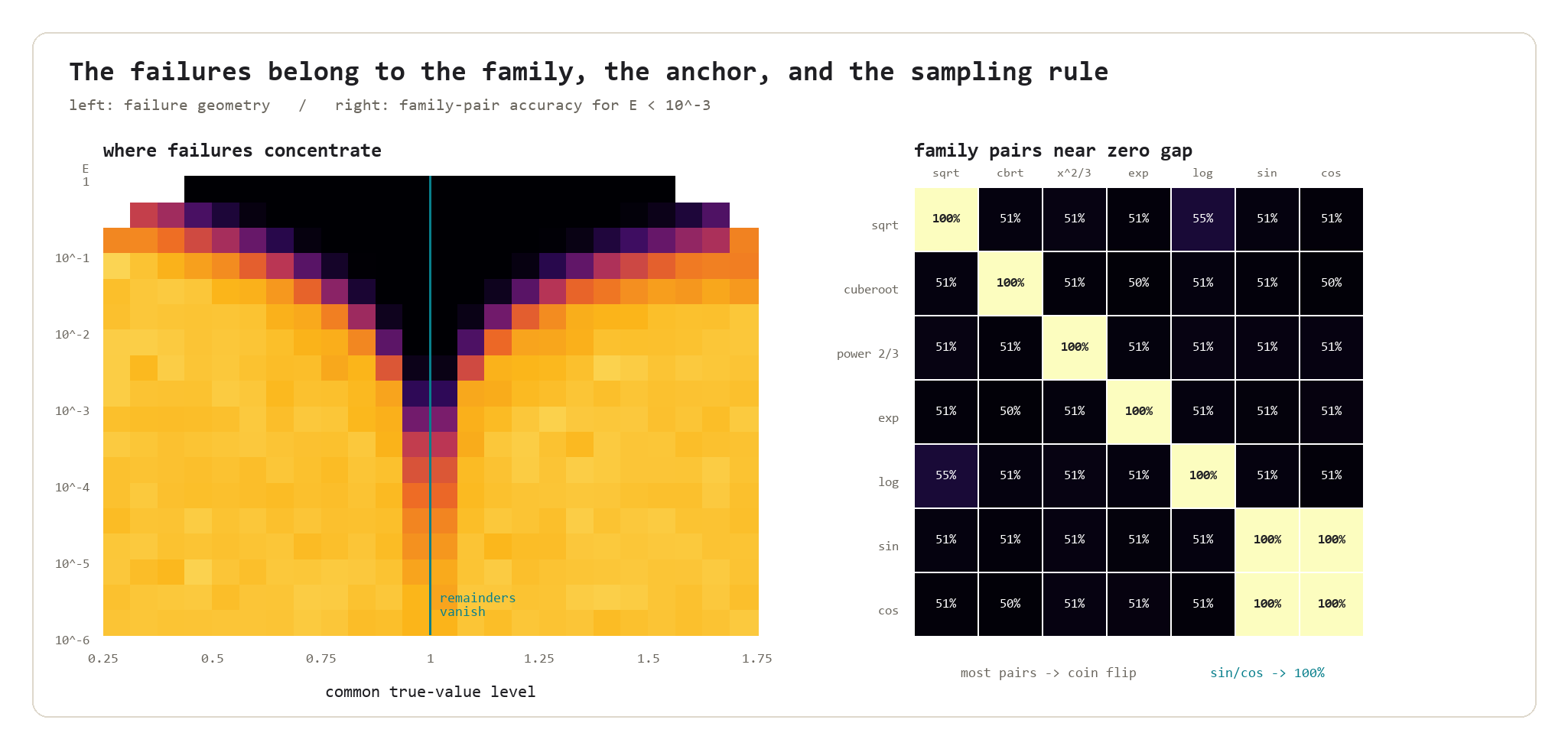
the family geometry is not background detail. it is the answer.
for \(x^a\) with \(0<a<1\), the function is increasing and concave, so the tangent sits above it. for \(e^x\), the tangent sits below it. for \(\log x\), it sits above again. these errors have direction; they are not random noise around zero.
then sin and cos can have stationary points where the first derivative becomes zero and the first-order approximation goes flat. now two distinct true values can get the exact same first-order value, which is a different failure mode entirely.
there is no single distance where “Taylor stops working”. the transition depends on the derivative, curvature, expansion point, branch, sampling rule, and most importantly the difference of the two remainders.
possible applications
the most obvious application is a cheap comparison filter.
suppose i want to know whether \(A>B\), but calculating either value accurately is expensive. i can first evaluate cheap approximations \(\hat A\) and \(\hat B\). if i also have remainder bounds
\[|r_A|\leq u_A, \qquad |r_B|\leq u_B,\]then the comparison is certified whenever
\[|\hat A-\hat B|>u_A+u_B.\]there is no need to compute more digits when the approximate gap is comfortably larger than the worst possible error. only the close cases need a better Taylor expansion, interval arithmetic, or exact evaluation.
this could be useful anywhere a numerical calculation eventually becomes a yes-or-no decision: choosing the larger of two candidates, deciding whether a constraint is active, comparing competing roots, or ranking approximate objective values in an optimization loop.
the important thing is that the approximation does not need to be uniformly good. it only needs to be reliable relative to the decision boundary. a method that is mediocre for reporting values might still be excellent for deciding which branch of an algorithm to take.
there is also a natural connection to computational geometry. many geometric algorithms repeatedly ask questions such as whether a point is to the left of a line, whether two quantities have crossed, or which of two intersections comes first. these are sign tests. a fast approximate predicate can handle the easy cases, while a slower and more reliable predicate is reserved for inputs near the boundary.
the probability curve gives a way to study that fallback rule empirically. if
\[p(E)=P(\text{correct ordering}\mid |A-B|\approx E),\]then a system could use the true-gap scale, or an estimate of it, to decide when first-order arithmetic is probably safe and when it should spend more work. that would not replace rigorous error bounds, but it could help benchmark different approximations and allocate precision where failures actually concentrate.
there is a broader lesson here for surrogate models too. a surrogate does not always need to reproduce the exact values of an expensive function. sometimes it only needs to preserve the ordering of nearby candidates. that is a weaker requirement in some regions and a much harder one in others, especially when the candidates are separated by less than the surrogate’s error.
so the practical question is not simply
how accurate is this approximation?
it is
accurate enough for which decision, at what separation, and with what fallback when the answer is uncertain?
that framing makes the strange Taylor examples feel less like curiosities. they are small versions of a very common numerical design pattern: use a fast approximate answer when the margin is large, detect when the margin is too small, and pay for accuracy only at the boundary.